Real-time visualisation of simulated lidar point-clouds with Mayavi and CARLA

This post shows how to visualise lidar point-clouds obtained from CARLA in real-time using the animation functionality from Mayavi. Although this post uses real-time data from CARLA, one can easily change the source of information to real sensors or simply replay recorded sensor data.

Motivation

CARLA provides a lidar visualisation script using Open3D available here. However, I personally found Open3D to have quite a long dependency list since it is a library for manipulating 3D data including an extensive list of algorithms. So I would rather use a tool created specifically for 3D data visualisation - enters Mayavi. Mayavi has a much smaller dependency list and is widely used to plot point clouds in the autonomous driving domain - usually adding bounding boxes to represent objects. However it comes with some perks, namely when creating visualisations for a continuous and asynchronous data stream. Since I could not find a better reference for this problem I decided to share my solution in this post.

CARLA Setup

Firstly, let’s set up the CARLA end to receive the data. This section assumes prior knowledge of the CARLA simulation environment and is partly adapted from PythonAPI/open3d_lidar.py

The first step is connecting with the CARLA server and setting up the synchronous mode, which will ensure that we get consistent point clouds.

import carla

client = carla.Client('localhost', 2000)
client.set_timeout(2.0)
world = client.get_world()

try:
	settings = world.get_settings()
	traffic_manager = client.get_trafficmanager(8000)
	traffic_manager.set_synchronous_mode(True)

	delta = 0.05

	settings.fixed_delta_seconds = delta
	settings.synchronous_mode = True
	settings.no_rendering_mode = arg.no_rendering
	world.apply_settings(settings)

Next we spawn an ego-vehicle into our simulated world using a random starting position and a random blueprint (vehicle model):

blueprint_library = world.get_blueprint_library()
vehicle_bp = blueprint_library.filter(arg.filter)[0]
vehicle_transform = random.choice(world.get_map().get_spawn_points())
vehicle = world.spawn_actor(vehicle_bp, vehicle_transform)
vehicle.set_autopilot(arg.no_autopilot)

We must now create our ray-cast lidar sensor and set-up some parameters (a complete list of sensor parameters is available here):

lidar_bp = blueprint_library.find('sensor.lidar.ray_cast')
lidar_bp.set_attribute('noise_stddev', '0.2')
lidar_bp.set_attribute('channels', str(64))                    #number of lasers, normally 64 or 128 (on newer lidar models).
lidar_bp.set_attribute('range', str(100))                      #range in meters
lidar_bp.set_attribute('rotation_frequency', str(1.0 / delta)) #ensures we will get a full sweep within a simulation frame

lidar_transform = carla.Transform(carla.Location(x=-0.5, z=1.8))
lidar = world.spawn_actor(lidar_bp, lidar_transform, attach_to=vehicle)
lidar.listen(lidar_callback)

The last line sets up the callback function that gets called everytime new data (point clouds) arrives, but we still do not know what this function should look like.

The simulation runs in synchronous mode in such a way that we must send a world.tick() event at every iteration step so that the simulation can run another loop iteration, updating the physical models and generating new sensor data. This prevents us getting flooded with data if our processing pipeline runs much slower than the simulation itself. Although the simulation runs in synchronous mode, the data is still transfered in an ansynchronous manner, which we receive through the callback function lidar_callback(data). To make sure the simulation runs continuously we create an infinite loop as

while True:
	time.sleep(0.005)
	world.tick()

We still need to figure out what the lidar_callback function looks like. This will depend on how we visualise our data, so now we dive into the Mayavi part!

Mayavi

Given a set of points pts with shape [N,3] where $N$ is the number of points and an optional set of intensities for each given point, one can visualise the point cloud using

from mayavi import mlab

#given a set of points pts [N,3] and a set of intensities [N,]
mlab.points3d(pts[:,0], pts[:,1], pts[:,2], intensity, mode='point')
mlab.show()

Given this, one could create the lidar callback function as

def lidar_callback(data):
  data = np.copy(np.frombuffer(point_cloud.raw_data, dtype=np.dtype('f4')))
  data = np.reshape(data, (int(data.shape[0] / 4), 4))

  #Isolate the intensity 
  intensity = data[:, -1]

  #Isolate the 3D data
  points = data[:, :-1]

  #We're negating the y to correclty visualize a world that matches
  #what we see in Unreal since Mayavi uses a right-handed coordinate system
  points[:, :1] = -points[:, :1]

  mlab.points3d(points[:,0], points[:,1], points[:,2], intensity, mode='point')
  mlab.show()

This creates a static visualisation each time a new packet of data arrives, which is quite inefficient and does not allow the user to interect with the data (i.e. change viewing angles). Mayavi provides a animation guide that shows how to create visualisations that change with time. However it assumes that the data is updated in synchronous intervals which is not the case when we obtain the data with a asynchronous callback function from an external source such as a simulation tool or a real sensor.

One way to solve this is to create a visualisation within the main thread scope (required by Mayavi) and update this visualisation once we get any callback with new data. This solution however requires calling mlab.show() on the main thread, which blocks the execution of code until the Mayavi visualisation screen is closed and means that we can no longer keep sending the world.tick() signals back to the simulator. To overcome this limitation we create a secondary thread that is responsible for sending the world.tick() updates, while at the same time creating an empty Mayavi visualisation window:

import threading

def carlaEventLoop(world):
  while True:
    time.sleep(0.005)
    world.tick()

loopThread = threading.Thread(target=carlaEventLoop, args=[world], daemon=True)
loopThread.start()

vis = mlab.points3d(0, 0, 0, 0, mode='point', figure=fig)
mlab.show()

Now one could implement the lidar callback function as

def lidar_callback(data, vis):
  data = np.copy(np.frombuffer(point_cloud.raw_data, dtype=np.dtype('f4')))
  data = np.reshape(data, (int(data.shape[0] / 4), 4))

  #Isolate the intensity 
  intensity = data[:, -1]

  #Isolate the 3D data
  points = data[:, :-1]

  #We're negating the y to correclty visualize a world that matches
  #what we see in Unreal since Mayavi uses a right-handed coordinate system
  points[:, :1] = -points[:, :1]

  #Update visualisation using Mayavi animation guide
  vis.mlab_source.reset(x=points[:,0], y=points[:,1], z=points[:,2], scalars=intensity)

#To register this callback we use a lambda function to mask the vis variable with the empty visualisation created previously
lidar.listen(lambda data: lidar_callback(data, vis))

This formulation tends to work most of the time, but occasionally fails with VTK errors such as Source array too small, requested tuple at index 11719, but there are only 11625 tuples in the array.. The error seems related to the frequency of updates created by the callback function. Although I did not have time to investigate why exactly this issue arises, I was able to come up with an alternative error-free solution.

The alternative solution consists of creating a buffer that stores the most recent point cloud received through the callback function, but only updating the Mayavi visualisation in synchronous intervals. The main part of the code (after creating the sensors and vehicle) looks like:

def lidar_callback(data, buf):
  data = np.copy(np.frombuffer(point_cloud.raw_data, dtype=np.dtype('f4')))
  data = np.reshape(data, (int(data.shape[0] / 4), 4))

  #Isolate the intensity 
  intensity = data[:, -1]

  #Isolate the 3D data
  points = data[:, :-1]

  #We're negating the y to correclty visualize a world that matches
  #what we see in Unreal since Mayavi uses a right-handed coordinate system
  points[:, :1] = -points[:, :1]

  #copy points/intensities into buffer
  buf['pts'] = points
  buf['intensity'] = intensity

def carlaEventLoop(world):
  while True:
    time.sleep(0.005)
    world.tick()

def main():
  #creates client,world ...
  #spawns vehicle ...
  #creates sensor ...

  #creates empty visualisation
  vis = mlab.points3d(0, 0, 0, 0, mode='point', figure=fig)
  #defines empty buffer
  buf = {'pts': np.zeros((1,3)), 'intensity':np.zeros(1)}
  #set callback
  lidar.listen(lambda data: lidar_callback(data, buf))

  #creates thread for event loop
  loopThread = threading.Thread(target=carlaEventLoop, args=[world], daemon=True)
  loopThread.start()

  #define mayavi animation loop
  @mlab.animate(delay=100)
  def anim():
      while True:
          vis.mlab_source.reset(x=buf['pts'][:,0], y=buf['pts'][:,1], z=buf['pts'][:,2], scalars=buf['intensity'])
          yield

  #start visualisation loop in the main-thread, blocking other executions
  anim()
  mlab.show()

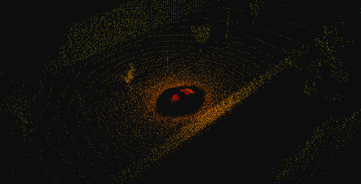
Visualisation results

Using the default lidar noise parameters for point dropout and Gaussian noise parameters we can now visualise the point clouds coming from the CARLA simulator in real time directly in the Mayavi interface:

Source code

You may find the complete code for this post in mayavi_lidar.py.